The previous post shows the difficulties to describe relational reality with the help of the limited concept of the “tangible” reality of the material world if the subject is related to the awareness of the human consciousness. So if we try to understand the part of relational reality that dominate consciousness (“live itself”) we have to search for useable (mathematical) concepts. At least we can give it a try.
The model of quantised space clarifies the general properties that physics has discovered with the help of experiments (the scientific method). The model explains the existence of the 2 universal conservation laws (energy and momentum), the universal constants (h and c) and some of the universal principles (non-locality and the uncertainty relation). The model also envelopes the general concept of quantum field theory (QFT), inclusive quantum gravity as an emergent vector field. But it also explains the origin of probability and even the non-Doppler red shift of the light of distant galaxies. Unfortunately these are clarifications that are not really helpful to understand “live itself”.
The model of quantised space is a mathematical model. That is why the model shows that the 1 : 1 relation between the universal electric field and its corresponding magnetic field in the primordial universe changed at the moment that rest mass emerged. The latter means that local concentrations of energy have forced scalars of the Higgs field to decrease their radius. The result is a further increase of the local concentration of energy what is known as rest mass carrying particles.
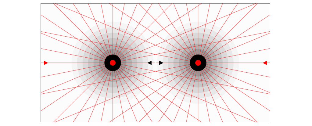
figure 1
However, decreased scalars interrupt the mediation of vectors by the flat Higgs field (vacuum space). But all the vectors in the universe are conserved (law of conservation of momentum). The consequence is that the interrupted part of a vector will become a displaced vector, like figure 1 shows (2 rest mass carrying particles). These displaced vectors will effect reality in an indirect way, comparable with the use of a side road instead of driving on the direct trajectory.
Unfortunately it is really hard to analyse how this indirect influence will manifest itself because vectors act instantaneous. That means that the position where the displaced vector will effect the energy of the universal electric field – actually the shape of the involved units of quantised space – is uncertain. Because if my focus is not the rest frame of quantised space, the interpretation of relational reality changes. If the displaced vector is thought to be the frame of reference, the metric of the rest frame becomes meaningless in relation to the position of the displaced vector.

figure 2
Every unit of quantised space without decreased scalar mediates vectors that arrive from adjacent scalars and passed on to other adjacent scalar. See the red scalar in figure 2. That means a distribution of vectors in relation to their direction and a distribution of vectors in relation to their magnitudes. The latter is restricted by the fixed amount of topological deformation of the unit. An amount of topological deformation that is directly related to the synchronisation of the deformation of all the units of quantised space during the constant of quantum time (1 tq). Actually, the synchronisation is responsible for the existence of the quantum of energy, the Planck constant (½ h for every single unit). The diameter of each scalar in figure 2 is about 0,5 x 10⁻¹⁵ m.
I have drawn a simplified partly transparent unit with the scalar vectors (black) pointing to the positions of the points of contact with the 12 adjacent scalars around (see figure 3). The red and green arrows symbolise the topological deformation of the related faces of the boundary of the unit at a certain moment. In other words, the real shape of the boundary of the unit is a deformed rhombic dodecahedron because the volume of every unit is invariant. The consequence is that the real surface area of the unit is larger than the surface area of the rhombic dodecahedron.
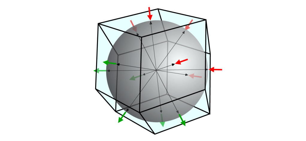
figure 3
If during 1 tq a unit deforms in a linear way – one red arrow and at the opposite side one green arrow – the velocity of the change is the speed of light. That makes it easy to understand energy configurations in nature. For example the resultant motion of “free” energy around a concentration of energy. Or the influence of energy density in relation to the properties of electromagnetic waves.
Unfortunately, trying to understand the existence of consciousness with the help of the properties of the corresponding vectors is quite confusing. It seems that there is no “tangible” relation between energy changes (universal electric field) and vectors that are supposed to “create” the awareness of consciousness. The latter means that a consciousness represents a certain volume that has at least slightly different properties than “vector space” (the flat Higgs field) around.
The sum of the change of the shape of the 12 faces of a unit during 1 tq can be expressed in terms of surface area and displaced volume. The latter is easier because the amount of volume of every unit is identical and also invariant (ΔVinput = ΔVoutput). In figure 3 the ΔVinput are the red arrows, the ΔVoutput are the green arrows).
The transfer of topological deformation between the units of quantised space is only possible if the total amount of surface area of all the individual units in the universe is conserved. In other words at the hypothetical “start” of the universe every unit of quantised space has a surplus of surface area in comparison with the amount of surface area of a rhombic dodecahedron with exactly the same volume. Surface area is energy (E = m c2) so it is obvious that the total surplus of surface area of all the units in the universe is conserved. The diagram in figure 4 shows the evolution of the asymmetrical energy distribution (the surplus of energy of the mass is equal to the deficit of the free energy in vacuum space).
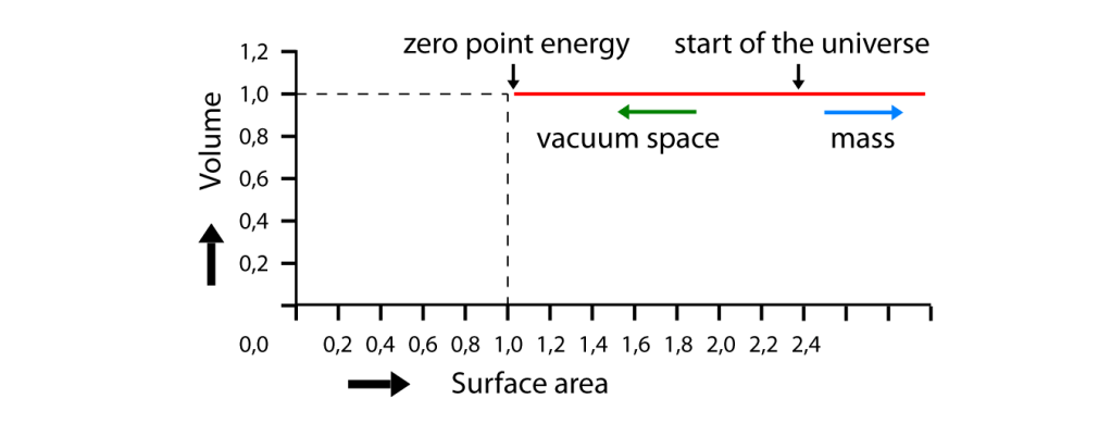
figure 4
In other words, if we focus on the total surface area (A) of one unit during 1 tq the equation is different (ΔA= ± 1 h). The consequence is that during 1 tq the sum of the magnitudes of the vectors corresponds with the change of the surface area of the unit. But the unit has 12 adjacent units. In other words, all the units of quantised space are forced to “individually” change their surface area with 1 h (input + output deformation). Now we can focus on the distribution of the change of surface area of the unit in relation to the change of the magnitudes of the vectors (v). That means Δv = (maps) h .
The schematic diagram in figure 5 shows the propagation of an electromagnetic wave in vacuum space. The wave form of the electric field (E) and the magnetic field (B) represent the spatial evolution in the x-direction of the influence of 1 h in relation to the electric and magnetic field around. That means that the transfer of 1 h by the electromagnetic wave is absorbed by the involved units around and than reversed, etc. Actually the waveform is the distribution of the vector and surface area (energy) of the Planck constant on the units around and the following reaction of the units around.
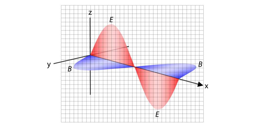
figure 5
The consequence is that every unit in the x-direction of the electromagnetic wave represents the evolving waveform during 1 tq. That means that the duration of the waveform in figure 5 is about 20 tq. So figure 5 shows the relevance of the synchronisation of all the changes of the units of quantised space, because without the synchronisation there is no waveform.
Figure 1 shows 2 rest mass carrying particles, the resultant vectors (red) around and the corresponding deformation of the electric field around the particles (concentric circles). Both particles interrupt vectors of the other particle. Vectors that are attached to the decreased scalar of the rest mass carrying particle.
We can observe the asymmetry with the help of experiments. Figure 6 shows the well known double slit experiment. If the slits are very small and close to each other in relation to the wave length of the electromagnetic wave the correspondence between the changes of the universal electric field and the vectors of the magnetic field get out of sync. The screen at the right shows the divergence.

figure 6
In other words, the difference between the velocity of the change of the shape of the units (c) tq) and the duration of the change of the corresponding vectors (instantaneous) results in local asymmetries of the correspondence. However, it also shows that the correspondence will “shape” the asymmetry. It is not reasonable to expect that a local surplus or deficit of related vectors will act as an independent phenomenon. The asymmetry is limited by the law of conservation of momentum and the principle of non-locality.
Conclusion
If the focus is on the change of energy we can visualise the change like the change is more or less an isolated occurrence (phenomenological point of view). Because the amount of change is a constant (h), the propagation is a constant (c) and the duration is a constant (tq). Although the related vectors reflect the change of energy (h), the influence of the vectors has not a clear position in relation to the structure of the units of quantised space. We cannot use the phenomenological point of view to visualise the changes within “vector space” because vectors non-local.
There is a continuous increase of matter in our universe. Therefore the amount of asymmetry of the correspondence between the universal electric field and the vectors of the magnetic field will not vanish. As long there is matter there will be local consciousness and the awareness of consciousness in relation to general consciousness.
